Spectral-shell representation

The spectral-shell representation is a physics-informed, low-dimensional projection of high-resolution stellar spectra designed to preserve information relevant to Doppler shifts and activity-driven line-profile variability. These notes review its development from the wavelength-gradient formulation of Cretignier et al. (2022), through the velocity-gradient and Doppler/shape-shell formulation of Zhao et al. (2024), to the information-weighted flux and formation-temperature representations of Gómez-Vargas et al. (2026). The emphasis is on mathematical construction, physical interpretation, methodological evolution, implementation, and assumptions.

Motivation and physical basis

Why compress the spectrum?

A high-resolution stellar spectrum is conventionally represented as normalized flux $f(\lambda)$. This contains essentially all spectral information, but a single spectrum can contain hundreds of thousands of pixels. Compressed observables such as the cross-correlation function (CCF) are easier to analyze, but averaging can suppress differences among spectral lines.

This matters for mitigating stellar activity. Different lines and different regions within a line react differently to magnetic activity because they probe different atmospheric depths. Suppression of convective blueshift in active regions modifies line depths, widths, and bisectors in a way that is not equivalent to a rigid translation of the entire spectrum.

The spectral shell occupies an intermediate regime:

$\text{full spectrum}\;\longrightarrow\;\text{spectral shell}\;\longrightarrow\;\text{CCF},$

with much lower dimensionality than the original spectrum while retaining more line-profile information than a CCF.

Linearized Doppler shift

Let $f_0(\lambda)$ be a high signal-to-noise master spectrum and $f(\lambda)$ an observed spectrum on the same wavelength grid. For a small displacement, a first-order Taylor expansion gives

$f(\lambda_i)-f_0(\lambda_i) = \frac{\partial f_0(\lambda_i)}{\partial\lambda_i}\,\delta\lambda_i.$

Define $\delta f_i = f(\lambda_i)-f_0(\lambda_i)$. Using the non-relativistic Doppler relation $\delta V_i/c=\delta\lambda_i/\lambda_i$, we obtain

$\boxed{\delta V_i = \frac{c}{\lambda_i}\,\delta f_i \left(\frac{\partial f_0(\lambda_i)}{\partial\lambda_i}\right)^{-1}.}$

To first order, the flux change produced by a pure Doppler shift is proportional to the local spectral gradient.

Why the spectral gradient matters

Pixels in a flat continuum have $\partial f_0/\partial\lambda\simeq 0$ and carry little first-order Doppler information. The same is true at the minimum of a symmetric absorption line. By contrast, the wings have large $\lvert\partial f_0/\partial\lambda\rvert$, and their opposite derivative signs distinguish the two sides. Thus $(f_0,\partial f_0/\partial\lambda)$ is a natural coordinate system for organizing pixels by their role inside absorption-line profiles.

Construction of the spectral shell

Original wavelength-gradient shell

Cretignier et al. (2022) introduced the shell as a projection onto $(f_0,\partial f_0/\partial\lambda)$. Each wavelength sample maps to

$\lambda_i\longmapsto \left(f_0(\lambda_i),\frac{\partial f_0(\lambda_i)}{\partial\lambda_i}\right).$

Wavelength is no longer an explicit shell coordinate. A single absorption line approximately traces a loop: the continuum approaches $(1,0)$, one wing has one gradient sign, the core has $f_0<1$ and nearly zero gradient, and the opposite wing has the opposite sign. Different lines can overlap when they occupy similar positions within their profiles.

Velocity-gradient shell

Zhao et al. (2024) reformulated the shell using the flux gradient in velocity space. Since $dv=(c/\lambda)\,d\lambda$, the chain rule gives

$\boxed{\frac{\partial f_0}{\partial v} =\frac{\lambda}{c}\frac{\partial f_0}{\partial\lambda}.}$

The Doppler relation simplifies to

$\boxed{\delta V_i=\delta f_i \left(\frac{\partial f_0(v_i)}{\partial v_i}\right)^{-1}, \qquad \delta f_i=\delta V_i\frac{\partial f_0(v_i)}{\partial v_i}.}$

This suppresses a dispersion-driven chromatic effect: similar line profiles at different wavelengths can have different wavelength gradients simply because of the factor $c/\lambda$. In velocity space, physically similar profiles approximately overlap in $(f_0,\partial f_0/\partial v)$ and share a common velocity scale.

Coordinates, stored quantity, and binning

The shell coordinates and the time-dependent quantity stored there are distinct. For each pixel,

$x_i=\left.\frac{\partial f_0}{\partial v}\right\rvert_{v_i}, \qquad y_i=f_0(v_i), \qquad z_i(t)=\delta f_i(t)=f(v_i,t)-f_0(v_i).$

The pair $(x_i,y_i)$ places the pixel; $z_i(t)$ carries its spectral variation. Conceptually,

$\mathcal{S}(x,y,t)\sim \delta f\!\left(f_0,\frac{\partial f_0}{\partial v},t\right).$

Discretizing the plane into cells $\mathcal{C}_{jk}$ yields a schematic shell cell

$S_{jk}(t)=\left\langle\delta f_i(t)\right\rangle_{i\in\mathcal{C}_{jk}}.$

The exact weighting or averaging depends on the implementation. The key operation is compression from roughly $N_\lambda\sim10^5$ pixels to $N_{\rm shell}\sim10^2$ cells.

Methodological evolution across the three papers

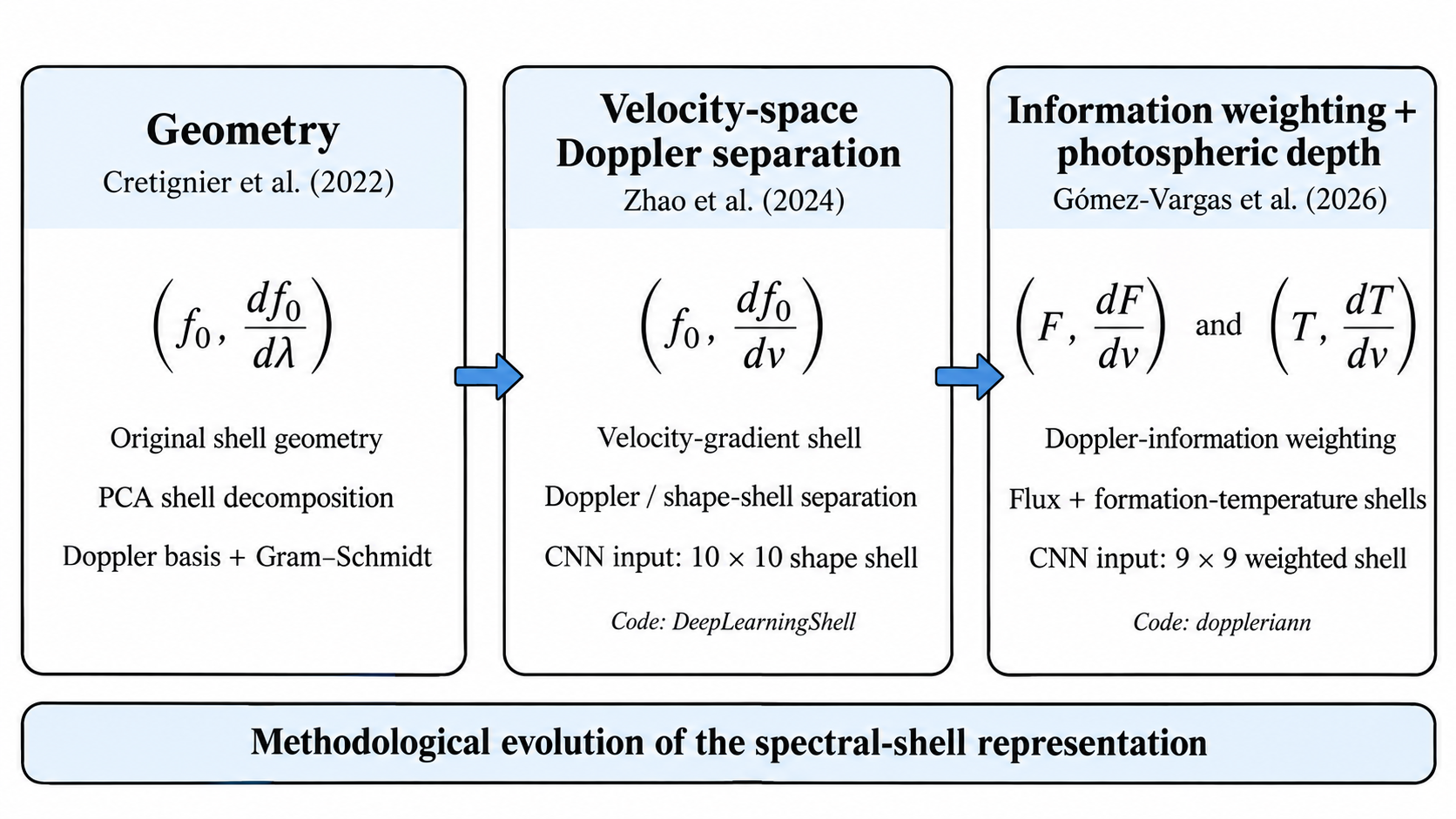
Evolution of spectral shells from wavelength-gradient geometry through velocity-space separation to information weighting and formation temperature

Evolution of the spectral-shell representation: wavelength-gradient geometry, velocity-space Doppler/shape separation, and information-weighted flux and formation-temperature shells.

Cretignier et al. (2022): shell geometry and PCA decomposition

Cretignier et al. define a binned shell in $(f_0,\partial f_0/\partial\lambda)$ space and use its time series to separate Dopplerian and non-Dopplerian variability. Principal-component analysis (PCA) produces a basis of non-Dopplerian shell variations. Because these components need not be orthogonal to the pure Doppler direction, a Gram–Schmidt step makes the basis orthogonal to the Doppler shell component:

$\delta f(t)=\alpha_{\rm DS}(t)\,\mathrm{DS} +\sum_{j=1}^{N}\alpha_j(t)\,\mathrm{PS}_j.$

Here $\mathrm{DS}$ is the pure-Doppler shell basis and $\mathrm{PS}_j$ are the orthogonalized principal shell components. The analysis uses YARARA post-processed spectra, after removal of major instrumental and telluric contaminants.

Zhao et al. (2024): velocity-gradient and shape shells

Zhao et al. move the shell to $(f_0,\partial f_0/\partial v)$ space. They select relatively clean, unblended lines deeper than approximately $0.1$ and bin the shell into a $10\times10$ array for their convolutional neural network (CNN).

A pure-Doppler template $S_{\rm Doppler}$ is generated by injecting a small Doppler shift into the master spectrum. After normalizing the template, the Doppler projection is $S_\parallel(t)=[S(t)\cdot S_{\rm Doppler}]S_{\rm Doppler}$. The Doppler-free shape shell is

$\boxed{S_{\rm shape}(t)=S(t)- \left[S(t)\cdot S_{\rm Doppler}\right]S_{\rm Doppler}.}$

This exposes activity-related line-shape variability while suppressing the direction in which a planetary signal should appear to first order. Code: DeepLearningShell.

Gómez-Vargas et al. (2026): information weighting and formation temperature

Gómez-Vargas et al. retain the velocity-gradient formalism and introduce a Doppler-information weight:

$\boxed{W_{v,i}=\left[\frac{\partial F_0(v_i)}{\partial v_i} \frac{1}{\sigma_{F_i}}\right]^2.}$

The cell weight is $W_{v,\mathrm{cell}}=\sum_{i\in\mathrm{cell}}W_{v,i}$ and the masked shell is formed element-wise: $S_{\rm masked}=S\odot W_v$.

The method extends normalized-flux space to formation-temperature space. Associate each pixel with an average formation temperature $T_{1/2}$ and construct a shell in

$\boxed{\left(T_{1/2},\frac{\partial T_{1/2}}{\partial v}\right).}$

For $g_T\equiv\partial T/\partial v$, the analogous velocity variation is $\Delta V_T=\Delta T/g_T$. Here $g_T$ is a numerical derivative of the temperature-valued spectrum along velocity, not a physical atmospheric temperature gradient such as $dT/dz$.

If flux uncertainty propagates to temperature uncertainty as $\sigma_T=f_{F\rightarrow T}(\sigma_F)$, then $\sigma_v=\sigma_T/g_T$ and

$\boxed{W^{(T)}_{v,i}= \left[\frac{g_{T,i}}{f_{F\rightarrow T}(\sigma_{F_i})}\right]^2.}$

The flux- and temperature-gradient shell spaces are both discretized into $9\times9$ grids in this implementation. Code: doppleriann, which includes flux and temperature shell construction, CCF/RV extraction, planetary injections, masking, detectability tests, and the deep-learning workflow.

Physical interpretation and comparison of shell variants

Pure Doppler motion versus line-shape variability

For a rigid Doppler displacement,

$\delta f_i=\delta V\frac{\partial f_0}{\partial v_i}.$

The entire spectrum follows one coherent direction in shell space. A line-depth change generally does not satisfy $\delta f_i/(\partial f_0/\partial v_i)=\text{constant}$. A bisector or asymmetry change affects the two wings differently because they occupy opposite signs of $\partial f_0/\partial v$. This is why shells help disentangle rigid shifts from stellar or instrumental line-shape perturbations.

Flux shell versus temperature shell

$\text{flux shell:}\quad\left(F_0,\frac{\partial F_0}{\partial v}\right), \qquad \text{temperature shell:}\quad \left(T_{1/2},\frac{\partial T_{1/2}}{\partial v}\right).$

The flux shell groups pixels by normalized line depth; the temperature shell groups them by an estimate of photospheric formation depth, designed to expose depth-dependent stellar variability more directly.

Geometric interpretation

The conventional spectrum maps $\lambda\mapsto f(\lambda)$. The shell maps each pixel to $(f_0(\lambda_i),\partial f_0/\partial v_i)$ and attaches its residual $\delta f_i(t)$ there. The question changes from “Where is this pixel in wavelength?” to “Where is this pixel within a line profile?”

Practical workflow, strengths, and limitations

Compact workflow

For each observation $f(\lambda,t)$:

Construct a high-S/N master spectrum $f_0(\lambda)$.
Compute $g_i=\left.\partial f_0/\partial v\right\rvert_i=(\lambda_i/c)\left.\partial f_0/\partial\lambda\right\rvert_i$.
Compute residuals $\delta f_i(t)=f_i(t)-f_{0,i}$.
Map selected pixels to shell coordinates $(f_{0,i},g_i)$ and bin the space into $S_{jk}(t)$.
Optionally calculate $W_{v,jk}=\sum_{i\in\mathcal{C}{jk}}[g_i/\sigma{F_i}]^2$ and form $S_{\rm masked}=S\odot W_v$.
In the Zhao et al. activity-mitigation formulation, remove the normalized Doppler direction to obtain the shape shell.
For temperature shells, replace $f_0$ with $T_{1/2}$ and $\partial f_0/\partial v$ with $\partial T_{1/2}/\partial v$, including the propagated uncertainties and weights.

Strengths

Strong dimensionality reduction relative to the native spectrum.
Retention of line-depth and asymmetry information partially averaged out by the CCF.
A mathematically explicit pure-Doppler direction.
Better comparability across wavelengths using the velocity gradient.
Compatibility with PCA and neural-network approaches.
Support for Doppler-information weighting and photospheric-depth information.

Limitations and assumptions

The small-shift derivation is first order and depends on a reference/master spectrum.
The compression is not generally bijective.
Blends and imperfect line selection can create degeneracies.
Shell resolution trades spatial detail against signal-to-noise.
Temperature shells require a reliable flux-to-formation-temperature mapping.
A fixed master spectrum does not explicitly encode all time-dependent activity-induced spectral changes.

Take-home synthesis: A spectral shell reorganizes wavelength pixels by their role within line profiles, making rigid Doppler motion simple and coherent while retaining non-Doppler line-shape information. The temperature extension additionally organizes that information by photospheric formation depth.

Code and data resources

The implementations discussed here include DeepLearningShell from Zhao et al. and doppleriann from Gómez-Vargas et al. The latter provides utilities for flux- and temperature-based shells, planetary Doppler injections, CCF-derived quantities, and neural-network training.

How the “density-weighted shell” is used

Shell and density are built together. In doppleriann/physics/spec_transform.py (lines 102 and 105), each bin stores mean residual flux and a density score (density_map).
Both arrays are saved in HDF5 datasets. doppleriann/data/shell_generation.py (lines 228–229) writes shells and density.
Weighting is applied when loading data. With use_mask=True, doppleriann/data/data_loader.py (line 339; documented at line 53) calculates $\mathbf{S}_{\mathrm{weighted}}=\mathbf{S}\odot\mathbf{D}$, where $\mathbf{D}$ is density.
Experiments generally enable this path. The scripts experiments/cnnShell_CV/cv5fold_cnn.py, cv_cnn_predict.py, and cv_cnn_detection.py set use_density_shell_mask=True (or use_mask=True).
Normalization preserves masked zeros. MaskedStandardScaler3D in doppleriann/data/scalers.py treats zeros as masked values during scaling.
This differs from KITCAT line weights. Multiplication by mask_weight[i] is commented out in doppleriann/physics/spec_transform.py (line 288), so KITCAT line weights are not applied there.

In this codebase, “weighted shell” therefore means the model input is typically $\mathbf{S}\odot\mathbf{D}$, enabled by use_mask=True during loading.

References

Cretignier, M., Dumusque, X., & Pepe, F. (2022). “Stellar activity correction using PCA decomposition of shells.” Astronomy & Astrophysics, 659, A68. doi:10.1051/0004-6361/202142435.
Zhao, Y., et al. (2024). “Improving Earth-like planet detection in radial velocity using deep learning.” Astronomy & Astrophysics, 687, A281. doi:10.1051/0004-6361/202450022.
Gómez-Vargas, I., Dumusque, X., Zhao, Y., Al Moulla, K., & Cretignier, M. (2026). “Modeling Doppler shifts in radial-velocity data with deep learning toward Earth-mass exoplanet detection.” Astronomy & Astrophysics, 712, A31. doi:10.1051/0004-6361/202659375.